Optimal Paths through Distribution Space for Mitigating Topological Freezing

Fisher geodesics and learned coupling fields in \(CP^{N-1}\)
The 43rd International Symposium on Lattice Field Theory

Roberto Dionisio

roberto.dionisio@phd.unipi.it

University of Pisa

July 27, 2026

Two flavors of critical slowing down

Standard critical slowing down:

\[\tau_{\mathrm{int}}(\mathcal{O}) \;\sim\; a^{-z}\]

Topological freezing: [1] [2]

\[\tau_{\mathrm{int}}(Q^2) \;\sim\; e^{\,c/a}\]

• Topology underlies key QCD phenomena:
  • Witten–Veneziano mechanism → \(m_{\eta'~}\)
  • Strong-CP problem (\(\theta\)-term)
  • QCD thermodynamics

How we can fight it?

Fighting freezing: an annealing protocol

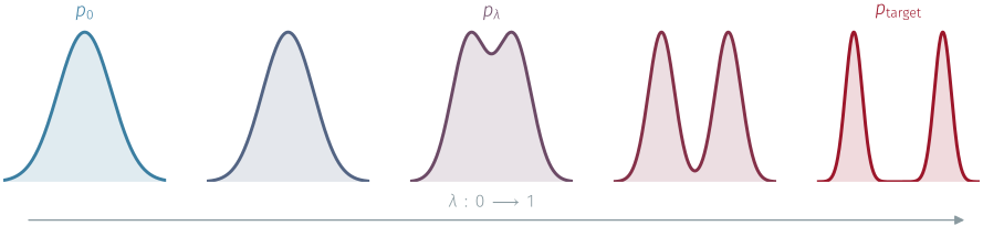
One route among others: interpolate an easy distribution to the target. [3]

\[S_\lambda = (1-\lambda)\,S_0 + \lambda\,S_{\mathrm{target}} \;\Longrightarrow \; p_\lambda \sim e^{-S_\lambda} \]

Learned sequential flows [6]

• NETS / Stochastic Normalizing Flows; [4] [5]
• sequential learned steps along \(\lambda\).

Parallel tempering

• parallel replicas exchanged along \(\lambda\);
• asymptotically exact, no network to train.

Fighting freezing: an annealing protocol

One route among others: interpolate an easy distribution to the target. [3]

\[S_\lambda = (1-\lambda)\,S_0 + \lambda\,S_{\mathrm{target}} \;\Longrightarrow \; p_\lambda \sim e^{-S_\lambda} \]

Learned sequential flows [6]

• NETS / Stochastic Normalizing Flows; [4] [5]
• sequential learned steps along \(\lambda\).

Parallel tempering

• parallel replicas exchanged along \(\lambda\);
• asymptotically exact, no network to train.

The testbed: 2D \(CP(N-1)\)

A QCD-like toy model
asymptotic freedom, a mass gap, \(\theta\)-vacua, and the same topological freezing

at a fraction of the cost.

Fundamental field: a unit complex \(N\)-vector

\[z(x)\in\mathbb{C}^N,\qquad z^{\dagger}(x)\,z(x)=1\]

with a local \(U(1)\) gauge redundancy

\[z(x)\;\longrightarrow\;e^{i\alpha(x)}\,z(x)\]

Lattice action:

\[S=-2N\beta\sum_{x,\mu}\mathrm{Re}\!\big[z^{\dagger}_x\,U_{x,\mu}\,z_{x+\hat\mu}\big]\]

Nontrivial topology:

\[\pi_2\!\big(CP^{N-1}\big)=\mathbb{Z}\]

Each configuration carries an integer topological charge

\[Q=\frac{1}{2\pi}\!\int\! d^2x\;\epsilon_{\mu\nu}\,\partial_\mu A_\nu\;\in\;\mathbb{Z}\]

Annealing the boundary: a tunable defect

Open BC [7]
No Topological barriers and \(Q\) change freely

Periodic BC
Target Physical Theory but topology is frozen!

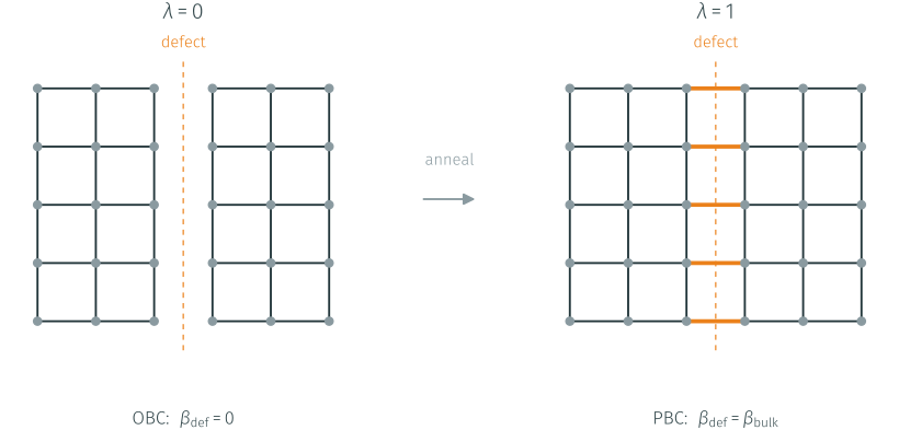
The defect is a line of links (a cut) with tunable coupling. [8]

Anneal \(\;\beta_{\mathrm{def}}(\lambda)=\lambda\,\beta_{\mathrm{bulk}}\): at \(\lambda=0\) the cut is open; at \(\lambda=1\) we recover the periodic theory.

Parallel tempering: a ladder of replicas

\(N_R\) replicas with fixed couplings \(\lambda_0=0\; ,\dots, \;\lambda_{N_R-1}=1\) run in parallel

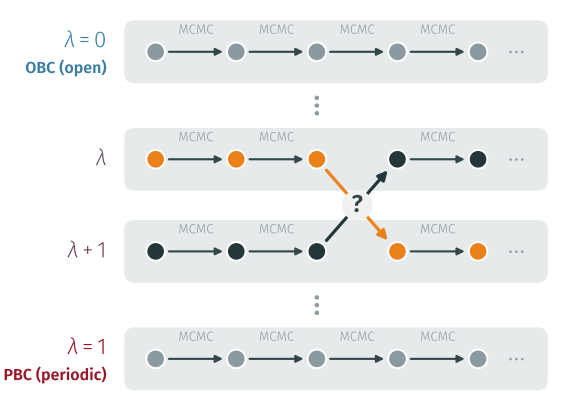
1. local MC in each replica samples its own \(p_\lambda\);

2. Propose a configuration swap between adjacent replicas

3. Accept/Reject \(\Longrightarrow\) detailed balance :

\(A=\min\!\big(1,\;\frac{p_{\lambda}(x_{\lambda+1})\, p_{\lambda+1}(x_{\lambda})}{p_{\lambda}(x_{\lambda})\, p_{\lambda+1}(x_{\lambda+1})}\big)\)

Efficient PT ladder \(\Longrightarrow\) topological mixing from the open replica to the target periodic one. [9]

Efficiency is a geometry problem

Given a fixed budget of steps / replicas, where should they go?

The answer comes from Information Geometry by studying the Fisher metric

Information geometry gives the answer

The space of probability distributions is a smooth manifold, carrying a natural metric \(\Rightarrow\) the Fisher metric:

\[g(\lambda) \;=\; \mathbb{E}_{p_\lambda}\!\Big[\big(\partial_\lambda \log p_\lambda\big)^2\Big]\]

For Boltzmann like \(p_\lambda \propto e^{-S_\lambda}\)

\[\partial_\lambda \log p_\lambda \;=\; -\,\partial_\lambda S_\lambda \;+\; \langle \partial_\lambda S_\lambda\rangle_{p_\lambda}\]

so the metric is just a variance:

\(g(\lambda) \;=\; \mathrm{Var}_{p_\lambda}\!\big[\partial_\lambda S_\lambda\big]\)

… and a distance

Second-order expansion of the KL divergence:

\[D_{\mathrm{KL}}\big(p_\lambda \,\|\, p_{\lambda+d\lambda}\big) \;\simeq\; \tfrac{1}{2}\, g(\lambda)\, d\lambda^2\]

\(g(\lambda)\) \(\Rightarrow\) local distinguishability of nearby distributions

large \(g\) \(\Rightarrow p_\lambda\) moves fast, hard to bridge small \(g\) \(\Rightarrow p_\lambda\) barely moves, easy

The geodesic condition

Thermodynamic length [10]
Fisher metric turns the path into a distance:

\[\Lambda \;=\; \int_0^1 \!\sqrt{g(\lambda)}\,d\lambda \left(=\; \sum_k \Delta\ell_k \right) \]

Running it in a finite (fictitious) time \(\tau\) dissipates work [11]

\[W_{\mathrm{diss}} \;\propto\; \frac{1}{\Delta t}\sum_k \Delta\ell_k^{\,2}\]

Minimize \(W_{\mathrm{diss}}\) at fixed length \(\Lambda\) leads to

\[\Delta\ell_1 \;=\; \Delta\ell_2 \;=\; \cdots \;=\; \Delta\ell_N .\]

\(\Delta\ell_k = \dfrac{\Lambda}{N} = \text{const} \;\;\Longleftrightarrow\;\; \dfrac{d\lambda}{dt}\propto\dfrac{1}{\sqrt{g(\lambda)}}\)

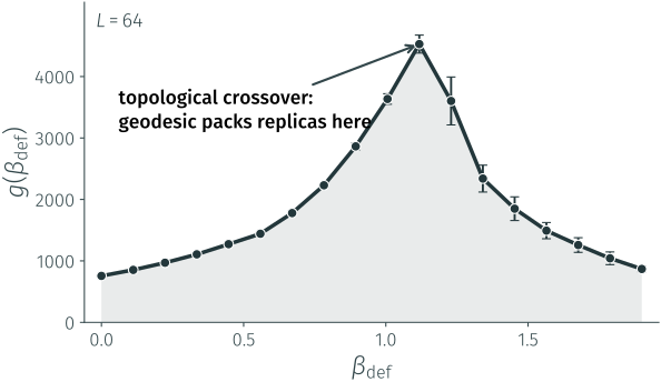
The geodesic condition:

1. Equidistribute the thermodynamic length

2. Spend more steps where \(g\) is large, fewer where it is small.

The protocol doesn’t have to be one-dimensional

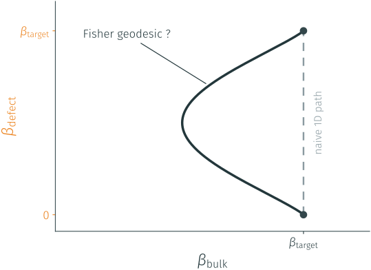
1. Let the bulk coupling vary along the path too:

\[g_{ij} \;=\; \mathrm{Cov}_{p}\!\big[\partial_{\beta_i} S,\; \partial_{\beta_j} S\big]\]

Optimal protocol \(\Rightarrow\) geodesic in the \((\beta_{\mathrm{bulk}},\,\beta_{\mathrm{defect}})\) plane.

2. The defect is local: it breaks translation invariance

Why hold every site to the same coupling?

Let it vary in space too:

\(\beta \;\longrightarrow\; \beta(x,y,t)\)

Learning the spatial coupling field

1 · Parametrize the field

\(d(x,y)\) → U-Net → \(F(x,y,\lambda)\)

\[\beta(x,y,\lambda) = \beta_{\mathrm{base}} + C_{\max}\,F(x,y,\lambda)\,\sin(\pi \lambda)\]

• \(\sin(\pi \lambda)\) pins the endpoints \(\lambda=0,1\);
• the net sees only geometry, i.e. distance to the defect, never field configurations \(\Rightarrow\) transferable

2 · The loss is the geometry

\[\begin{aligned} \mathrm{sKL}(p_r, p_{r+1}) &= \tfrac{1}{2}\big[\,D_{\mathrm{KL}}(p_r \,\|\, p_{r+1}) + D_{\mathrm{KL}}(p_{r+1} \,\|\, p_r)\,\big] \\[3pt] &= \tfrac{1}{2}\big[\langle \Delta S\rangle_{p_r} - \langle \Delta S\rangle_{p_{r+1}}\big] \end{aligned}\]

Small steps: \(\;\mathrm{sKL}_r \approx \tfrac{1}{2}\,g(\lambda_r)\,\Delta\lambda_r^{2} = \tfrac{1}{2}\,\Delta\ell_r^{2}\)

\[\sum_r \mathrm{sKL}_r \;\approx\; \tfrac{1}{2}\sum_r \Delta\ell_r^{2}\;\ge\;\frac{\Lambda^{2}}{2N}\]

Minimizing it \(\Rightarrow\) equal \(\Delta\ell\):

Geodesic of length \(\Lambda\), from PT samples (no \(Z\)).

Parallel tempering
sampling

\(\beta(x,y,\lambda)\) →

← \(\nabla\,\mathrm{sKL}\)

Network
update

The U‑Net learns the Fisher geodesic end‑to‑end from PT samples,does its trajectory match the theory?

The model finds the geometry

\(L=32 \quad \beta=1.8 \quad N=6\)

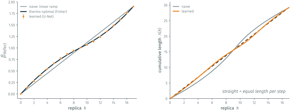
The learned schedule lands
on the measured Fisher optimum.

…and walks it at equal thermodynamic length per step
the geodesic condition recovered from samples alone.

Solved ladder bottleneck

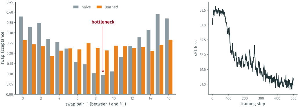
The naive ladder drops to 9.5% acceptance at the crossover.
The learned schedule keeps every bin uniform, so replicas round-trip.

It gets there by minimizing the sKL loss — equal-length steps, the geodesic condition.

A field of coupling

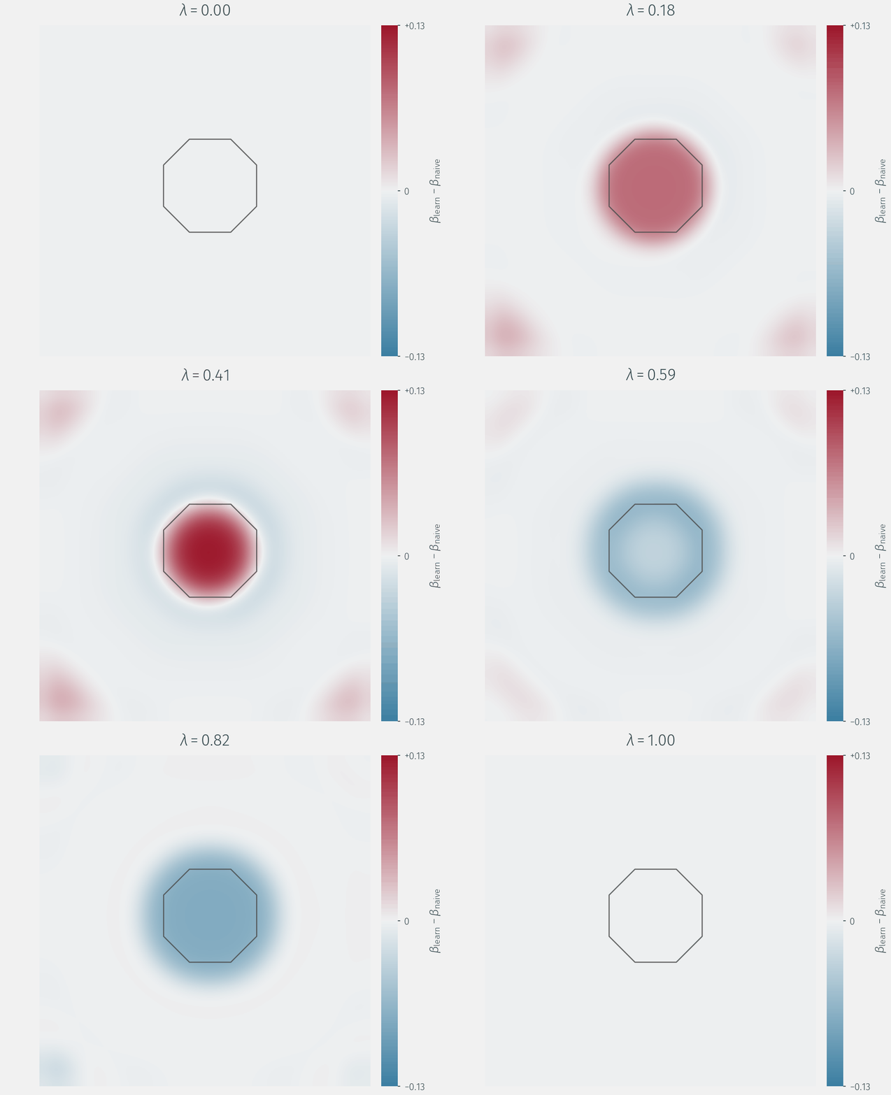
The U-Net emits a full field \(\beta(x,y,\lambda)\);
not a scalar schedule.

• early: drives the defect coupling ahead of the ramp;
• late: holds it back;

Freedom no scalar schedule has.

• We have explored different defect shapes: disk, square and stripe
• We stick to a finite stripe (cheaper).

Topology is not frozen!

\(N=21 \quad L=150 \quad \beta \simeq 0.8 \quad N_R=12\)

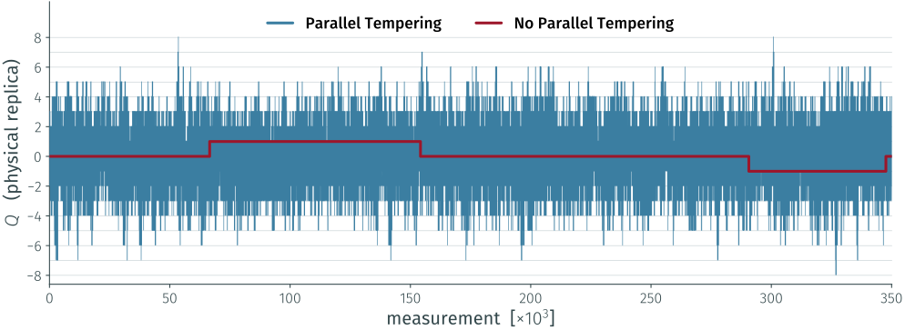
The full run ~350k measurements (\(L=150\), optimized schedule): the physical replica visits sectors \(-8\ldots+8\).
Tempering through the defect keeps the charge unfrozen, where local updates would freeze it.

Critical slowing down of Q²

\(\tau_{\mathrm{int}}(Q^2)\sim(\xi/a)^{z}\)

\(\Lambda/\xi \equiv L_d/\xi \qquad\) \(\qquad L_d \lesssim 12\%\,L \qquad\) \(\qquad \Lambda \propto \sqrt{L_d} \qquad\)

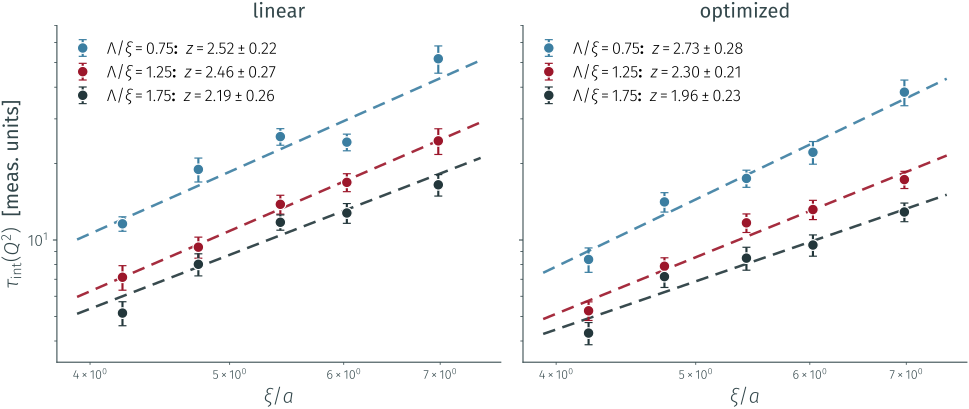
Five volumes with \(L/\xi \gtrsim 20\) and three defect sizes: optimized schedule (right) sits systematically below the linear one (left).

Optimized annealing pays off

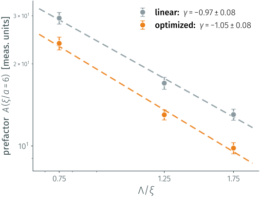
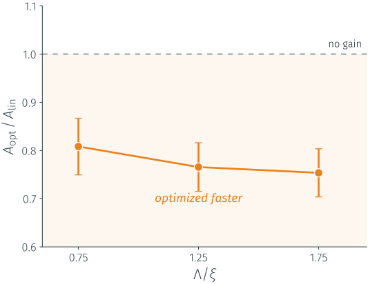
The prefactor falls as \(A\sim(\Lambda/\xi)^{\gamma}\) with \(\gamma\approx-1\)
a larger defect (more replicas) already helps.

On top of that, the optimized schedule has a further \(\sim20\%\) off, uniformly in \(\Lambda/\xi\).

Conclusions

Parallel tempering + optimal schedule beats topological freezing

With the Fisher-geodesic condition we get a good diffusion of topological mixing, from the open replica up to the periodic one.

A ready-made, exact framework

The same parallel tempering already runs in full \(2\!+\!1\) QCD [9], and across 2D CP(N-1) [12][13] and pure-gauge SU(3) / SU(N) [14][15][16]. Schedule optimization plugs straight in.

Outlook · minimize the cost, not only the protocol: a cost function of the defect size \(L_d\), the number of replicas \(N_R\) and the autocorrelation time \(\tau_{\mathrm{int}}\), minimized to the true compute optimum.

Thank you for your attention!

References

[1] Del Debbio, Manca, Vicari, Phys. Lett. B 594 (2004) 315 [arXiv:hep-lat/0403001]
[2] Schaefer, Sommer, Virotta (ALPHA), Nucl. Phys. B 845 (2011) 93 [arXiv:1009.5228]
[3] Neal, Stat. Comput. 11 (2001) 125 [arXiv:physics/9803008]
[4] Caselle, Cellini, Nada, Panero, JHEP 07 (2022) 015 [arXiv:2201.08862]
[5] Albergo, Vanden-Eijnden, ICML 2025 [arXiv:2410.02711]
[6] Albergo, Kanwar, Shanahan, Phys. Rev. D 100 (2019) 034515 [arXiv:1904.12072]
[7] Lüscher, Schaefer, JHEP 07 (2011) 036 [arXiv:1105.4749]
[8] Hasenbusch, Phys. Rev. D 96 (2017) 054504 [arXiv:1706.04443]
[9] Bonanno, Clemente, D’Elia, Maio, Parente, JHEP 08 (2024) 236 [arXiv:2404.14151]
[10] Crooks, Phys. Rev. Lett. 99 (2007) 100602 [arXiv:0706.0559]
[11] Sivak, Crooks, Phys. Rev. Lett. 108 (2012) 190602 [arXiv:1201.4166]
[12] Berni, Bonanno, D’Elia, Phys. Rev. D 100 (2019) 114509 [arXiv:1911.03384]
[13] Bonanno, Phys. Rev. D 107 (2023) 014514 [arXiv:2212.02330]
[14] Bonanno, Dasilva Golán, D’Elia, García Pérez, Giorgieri, EPJC 84 (2024) 916 [arXiv:2403.13607]
[15] Bonanno, JHEP 01 (2026) 039 [arXiv:2510.08006]
[16] Bonanno, Bonati, D’Elia, JHEP 03 (2021) 111 [arXiv:2012.14000]

Where the exponential comes from

Particle on a ring

\(x(\tau): S^1_\tau \rightarrow S^1_x\)

The path integral splits into homotopy sectors by winding number \(Q\in\mathbb{Z}\):

\[Z \;=\; \sum_{Q} Z_Q\]

Local Algorithms:

Constant acceptance ⇒ \(\delta x \sim \sqrt{a}\).

Topology changes require crossing an action barrier \(\Delta S \sim c/a\)

\(P_{\mathrm{tunnel}} \sim e^{-\Delta S} \quad\Longrightarrow\quad \tau_{\mathrm{int}}(Q) \sim e^{\,\Delta S} \sim e^{\,c/a}\)

Particle on a ring: the path integral splits into homotopy classes labelled by the winding number Q (pi_1(S^1) = Z); the two boxes are the Q=0 and Q=+1 sectors. Local Monte Carlo at fixed acceptance proposes path changes of order sqrt(a). Changing Q needs a defect – one link with Dphi ~ pi – costing DS ~ 1/a ~ 2 beta-tilde, a barrier that diverges in the continuum. Tunnelling is suppressed as e^{-DS}, so tau_top ~ e^{c/a}. Same mechanism in CP^(N-1) and QCD.